Transmission spectra

General transmission spectra

In this section we’ll use the general transmission spectrum model from de Wit & Seager (2013). We will compute the transmission spectrum for an Earth-sized planet, for an atmosphere in chemical equilibrium, using only the opacities for water and carbon dioxide.

First we will import the necessary packages, and choose the wavelengths, temperatures, and pressures:

import numpy as np
import matplotlib.pyplot as plt
import astropy.units as u
from astropy.constants import G

from jax import numpy as jnp

from shone.chemistry import FastchemWrapper, species_name_to_fastchem_name
from shone.opacity import Opacity
from shone.transmission import de_wit_seager_2013

wavelength = np.geomspace(0.5, 5, 500)
pressure = np.geomspace(1e-6, 1)  # [bar]
temperature = 700 * (pressure / 0.1) ** 0.05  # [K]

Load opacities

Let’s load those opacities from the demo opacities with load_demo_species:

opacity_samples = []
molecules = ['H2O', 'CO2']
for molecule in molecules:

    # in this example we'll use the demo opacities,
    # which you *should not use* in real work:
    opacity = Opacity.load_demo_species(molecule)
    interp_opacity = opacity.get_interpolator()
    opacity_samples.append(
        interp_opacity(wavelength, temperature, pressure)
    )

total_opacity = jnp.array(opacity_samples).sum(axis=0)

Let’s see where each species contributes to the opacity:

ax = plt.gca()

for molecule, op in zip(molecules, opacity_samples):
    ax.semilogy(
        wavelength, op[30],
        label=molecule.replace('2', '$_2$')
    )

plt.legend()
ax.set(
    xlabel='Wavelength [µm]',
    ylabel='Opacity [cm$^2$ g$^{-1}$]',
    ylim=(1e-6, 1e5)
)

(Source code, png)

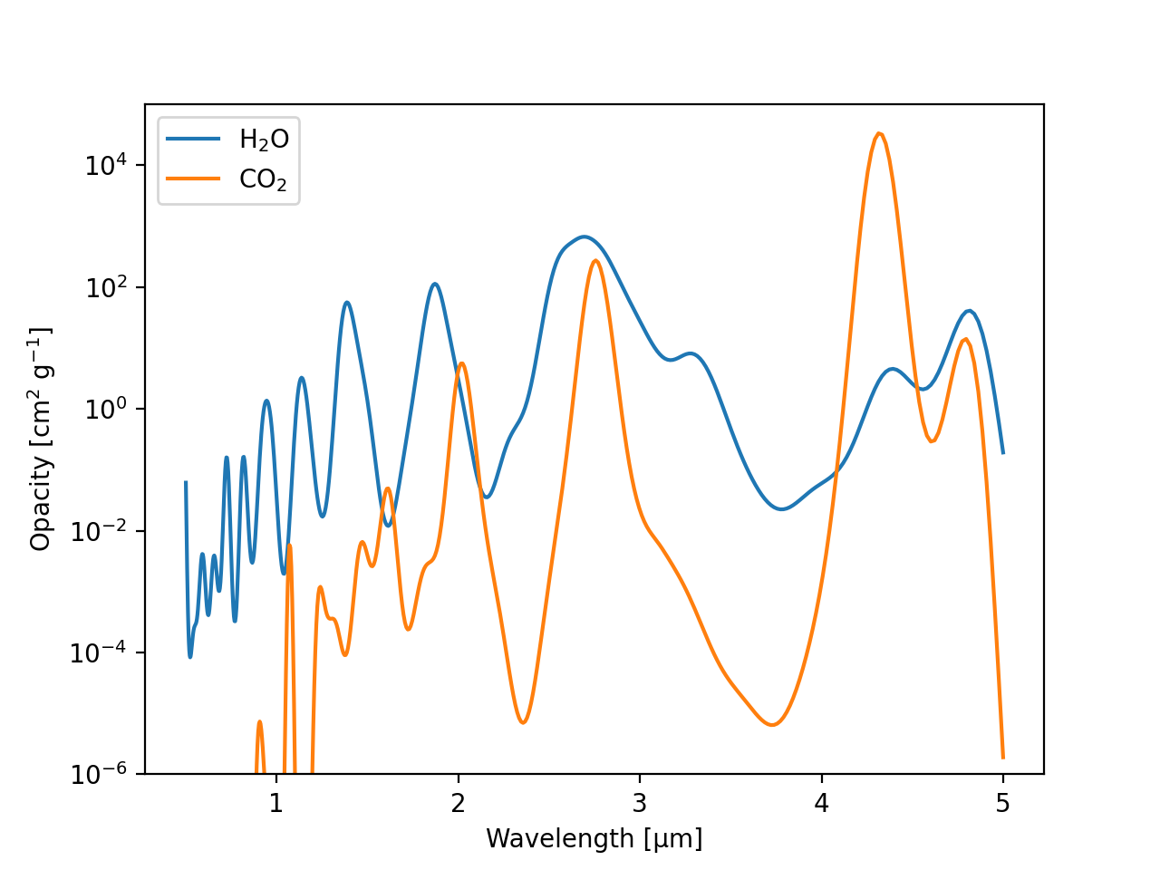
Warning

These demo opacities are meant for documentation and testing only, and are not reliable near either wavelength limit in this plot, or at very low opacities. For more background on these tiny opacity archives, see Tiny opacity archives.

Equilibrium chemistry

We compute the volume mixing ratios in chemical equilibrium from FastChem via FastchemWrapper:

chem = FastchemWrapper(temperature, pressure)
vmr = chem.vmr()
weights_amu = chem.get_weights()

vmr_indices = chem.get_column_index(species_name=molecules)

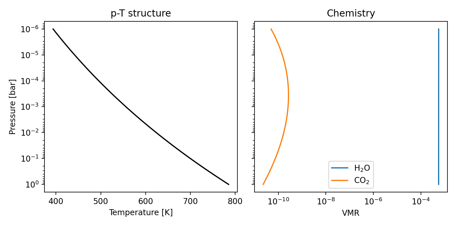
Let’s see what the mixing ratios are as a function of pressure:

fig, ax = plt.subplots(1, 2, figsize=(8, 4), sharey=True)

ax[0].semilogy(temperature, pressure, color='k')
ax[0].set(
    xlabel='Temperature [K]',
    ylabel='Pressure [bar]',
    title='p-T structure'
)
ax[0].invert_yaxis()

for molecule, vmr_i in zip(molecules, vmr[:, vmr_indices].T):
    ax[1].loglog(vmr_i, pressure, label=molecule.replace('2', '$_2$'))
ax[1].legend()
ax[1].set(
    xlabel='VMR',
    title='Chemistry'
)
plt.tight_layout()

(Source code, png)

Compute transmission

In order to know the planetary surface gravity, and to compute the ratio of the planetary to stellar radii, we need to specify some system parameters:

R_p0 = (1 * u.R_earth).cgs.value  # [cm]
mass = (1 * u.M_earth).cgs.value  # [g]
g = (G * mass / R_p0**2).cgs.value  # [cm/s2]
R_star = (1 * u.R_sun).cgs.value  # [cm]

Now we bring all of the pieces together in transmission_radius and plot the result:

# compute the transmission spectrum:
Rp_Rs = de_wit_seager_2013.transmission_radius(
    wavelength, temperature, pressure,
    g, R_p0,
    total_opacity[None, ...],
    vmr, vmr_indices, weights_amu,
    rayleigh_scattering=True
) / R_star

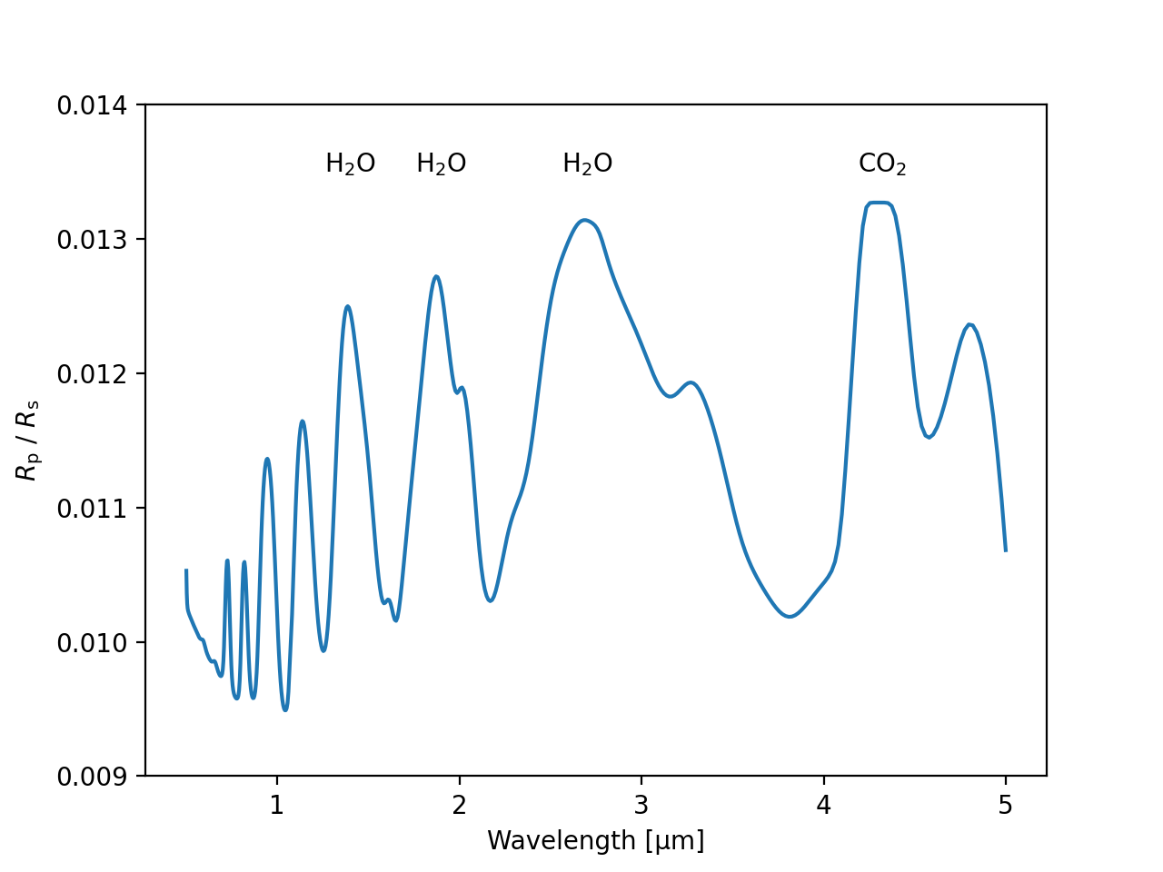
# plot transmission spectrum:
ax = plt.gca()
ax.plot(wavelength, Rp_Rs)

# add labels for CO2 and H2O features:
label_height = 0.0135
ax.annotate("CO$_2$", (4.32, label_height), ha='center')

water_peaks = [1.4, 1.9, 2.7]
for peak in water_peaks:
    ax.annotate("H$_2$O", (peak, label_height), ha='center')

ax.set(
    xlabel='Wavelength [µm]',
    ylabel='$R_{\\rm p}~/~R_{\\rm s}$',
    ylim=(0.009, 0.014)
)

(Source code, png)

We’ve labeled prominent absorption features from water and carbon dioxide, and you can see the upturn at short wavelengths due to Rayleigh scattering.

Isothermal/isobaric transmission spectra

Let’s compute the transmission spectrum for an Earth-like planet with a single-species atmosphere using the isothermal and isobaric approximations from Heng & Kitzmann (2017). The full transmission model is demonstrated above in General transmission spectra.

We’ll load an opacity grid and interpolate for the opacity at several temperatures, add a gray cloud opacity, and compute a transmission spectrum.

Load opacity

Note

This example uses a synthetic opacity file that is totally made up. To download real opacity grids, see Opacities.

Let’s synthesize a transmission spectrum for an Earth-sized planet with one atmospheric species in the near-infrared.

import numpy as np
from jax import numpy as jnp, jit
import matplotlib.pyplot as plt

import astropy.units as u
from astropy.constants import m_p

from shone.opacity import Opacity, generate_synthetic_opacity
from shone.transmission import heng_kitzmann_2017

For each species to include in the atmosphere, you need to download an opacity grid for that species. We load and interpolate opacity grids using the Opacity class. For this example, we’ll use a synthetic opacity grid, generated with by function:

generate_synthetic_opacity()

We can check which species are already chached and available on your machine using get_available_species():

Opacity.get_available_species()

Table length=9

name	species	charge	line_list	path	index
synthetic	synthetic	--	example	/Users/bmmorris/.shone/synthetic__example.nc	0

Let’s load the opacity file named “synthetic” that we created above:

# load the synthetic opacity file:
opacity = Opacity.load_species_from_name('synthetic')

Interpolating opacities

Now we will create a just-in-time compiled opacity interpolator. get_interpolator returns a function that takes three arguments – a wavelength array [µm], a temperature [K], and a pressure [bar] – and returns an array of opacities for each wavelength:

# get a jitted 3D interpolator over wavelength, temperature, pressure:
interp_opacity = opacity.get_interpolator()

Let’s compute the opacity at one temperature and pressure:

wavelength = np.linspace(1, 5, 500)  # [µm]
pressure = 1  # [bar]
temperature = 200  # [K]

example_opacity = interp_opacity(wavelength, temperature, pressure)

plt.semilogy(wavelength, example_opacity, label=f"T={temperature} K")
plt.legend()
plt.gca().set(
    xlabel='Wavelength [µm]',
    ylabel='Opacity, $\kappa$ [cm$^2$ g$^{-1}$]'
)

(Source code, png)

Now let’s specify an opacity for a gray cloud:

kappa_cloud = 5e-2  # [cm2/g]

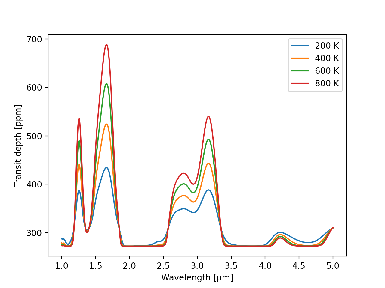
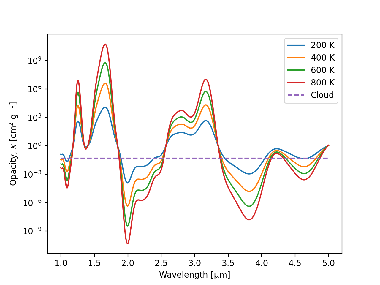
Suppose we want to compute transmission spectra for several atmospheric temperatures:

# interpolate for a range of wavelengths at one pressure and temperature:
temperature = np.array([200, 400, 600, 800])  # [K]
pressure = np.ones_like(temperature)  # [bar]

example_opacity = interp_opacity(wavelength, temperature, pressure)

and now let’s plot the result:

label = [f"{t} K" for t in temperature]

plt.figure()
plt.semilogy(wavelength, example_opacity.T, label=label)
plt.semilogy(wavelength, kappa_cloud * np.ones_like(wavelength), ls='--', label="Cloud")
plt.legend()
plt.gca().set(
    xlabel='Wavelength [µm]',
    ylabel='Opacity, $\kappa$ [cm$^2$ g$^{-1}$]'
)

(Source code, png)

Compute transmission

We can compute a transmission spectrum for an Earth-sized planet transiting a Sun-like star using transmission_radius_isothermal_isobaric:

R_0 = 1 * u.R_earth  # reference radius
P_0 = 1 * u.bar  # reference pressure
T_0 = 290 * u.K  # reference temperature
mmw = 28 * m_p  # mean molecular weight (AMU)
g = 9.8 * u.m / u.s**2  # surface gravity

# convert the arguments from astropy `Quantity`s to
# floats in cgs units:
args = (R_0, P_0, T_0, mmw, g)
cgs_args = (arg.cgs.value for arg in args)

# compute the planetary radius as a function of wavelength:
Rp = heng_kitzmann_2017.transmission_radius_isothermal_isobaric(
    example_opacity + kappa_cloud, *cgs_args
)

# convert to transit depth:
Rstar = (1 * u.R_sun).cgs.value
transit_depth_ppm = 1e6 * (Rp / Rstar) ** 2

Now let’s plot the result:

label = [f"{t} K" for t in temperature]
plt.plot(wavelength, transit_depth_ppm.T, label=label)
plt.legend()
plt.gca().set(
    xlabel='Wavelength [µm]',
    ylabel='Transit depth [ppm]'
)

(Source code, png)