Opacities

Download opacities

Several helper methods are included in shone for downloading and archiving local copies of opacities stored on DACE via the package dace-query. Users can access the DACE API without any special registration, though a warning will appear saying “File .dacerc not found. You are requesting data in public mode…” If you like, you may register for an API key to use dace-query, see their documentation for instructions.

To download the opacities for an atom with download_atom(), specify the atom’s name and charge, and optionally limit the pressure range (in log10 bars) and temperature range (in Kelvin):

from shone.opacity.dace import download_atom

download_atom(
    atom='Na',
    charge=0,
    temperature_range=[2500, 2500]
)

You may query for molecules by their common names (for the most common isotopologue) with download_molecule() like so:

from shone.opacity.dace import download_molecule

download_molecule(
    molecule_name='H2O',
    temperature_range=[2500, 2500],
    pressure_range=[-6, -6]
)

or for a specific isotopologue:

from shone.opacity.dace import download_molecule

download_molecule(
    isotopologue='1H2-16O',
    temperature_range=[2500, 2500],
    pressure_range=[-6, -6]
)

These methods download the opacity grids from DACE, and store them in a netCDF file in your home directory with the name .shone/.

Example opacity file

It is often useful to have a small, synthetic opacity file for simple demos and testing. You can generate one with generate_synthetic_opacity():

from shone.opacity import generate_synthetic_opacity

opacity = generate_synthetic_opacity()

You can also lookup and load opacities within the cache like so:

from shone.opacity import Opacity

# load the one opacity file:
opacity = Opacity.load_species_from_name('synthetic')

Opening opacities

Opacities are loaded and interpolated with the Opacity class:

from shone.opacity import Opacity

We can check which species are already chached and available on your machine using get_available_species():

Opacity.get_available_species()

This will return a table of available opacity grids on disk.

Let’s load the opacity created by generate_synthetic_opacity() (see the step above):

opacity = Opacity.load_species_from_name('synthetic')

The Opacity object contains the opacity grid as a DataArray in its grid attribute. You can see the dimensions of the grid with:

>>> print(opacity.grid.coords)
Coordinates:
  * wavelength   (wavelength) float64 0.5 0.5012 0.5023 ... 4.977 4.988 5.0
  * temperature  (temperature) int32 200 400 600 800 1000
  * pressure     (pressure) float64 1e-06 10.0

The coordinates in the DataArray are wavelength in microns, temperature in K, and pressure in bar. To learn to use the xarray API directly on the grid attribute, refer to the xarray docs on indexing and selecting data and interpolating.

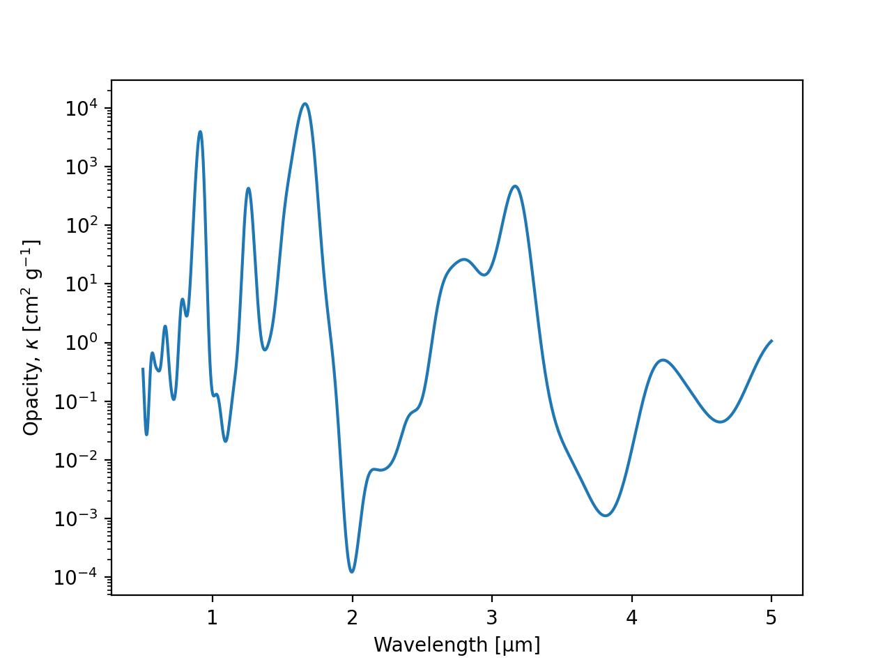
You can inspect the opacities from one temperature and pressure slice like so:

import matplotlib.pyplot as plt

opacity_sample = opacity.grid.sel(
    dict(
        pressure=10,  # [bar]
        temperature=200  # [K]
    )
)

plt.semilogy(
    opacity_sample.wavelength, opacity_sample,
    label=f"T={opacity_sample.temperature} K"
)
plt.gca().set(
    xlabel='Wavelength [µm]',
    ylabel='Opacity, $\kappa$ [cm$^2$ g$^{-1}$]'
)

(Source code, png)

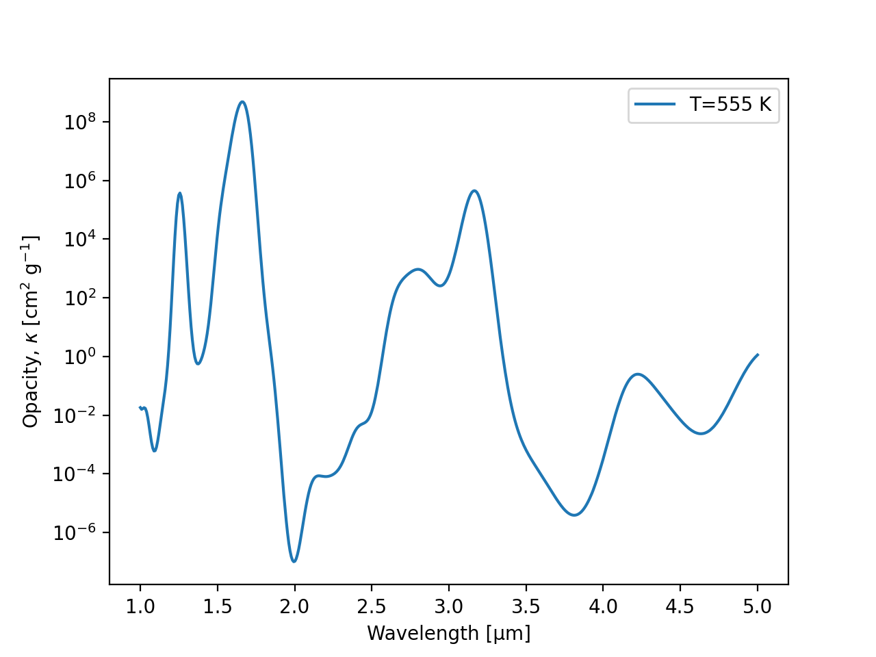
Interpolating opacities

Often in shone we will need to interpolate over the opacity grid within compiled code, so we will use a just-in-time compiled interpolator on the opacity grid. You can produce a function to do these compiled interpolations with get_interpolator:

# get a jitted 3D interpolator over wavelength, temperature, pressure:
interp_opacity = opacity.get_interpolator()

Now you can get the opacity at wavelengths, temperatures, and pressures that weren’t on the grid:

import numpy as np
import matplotlib.pyplot as plt

wavelength = np.linspace(1, 5, 500)  # [µm]
pressure = 0.3  # [bar]
temperature = 555  # [K]

example_opacity = interp_opacity(wavelength, temperature, pressure)

plt.semilogy(wavelength, example_opacity, label=f"T={temperature} K")
plt.legend()
plt.gca().set(
    xlabel='Wavelength [µm]',
    ylabel='Opacity, $\kappa$ [cm$^2$ g$^{-1}$]'
)

(Source code, png)

We can compute opacities over a series of temperatures and pressures:

from jax import numpy as jnp

temperatures = jnp.array([222, 333, 444])
pressures = jnp.array([0.1, 0.5, 0.9])

example_opacity = interp_opacity(wavelength, temperatures, pressures)

For M wavelengths and N samples in pressure and temperature, the output will have the shape (N, M).

Crop an opacity grid

Suppose the full opacity grid covers a wider wavelength range than you need for your calculation. You can limit the size of the array that gets read into JAX by cropping the opacity grid to the relevant limits in wavelength, pressure, and temperature.

The example opacity file above is small compared to real ones, and contains this many opacity entries:

>>> print(opacity.grid.size)
10000

To reduce the size of the opacity grid, we crop the opacity grid on the wavelength range \(1.5 < \lambda < 2.5\) µm:

crop = ((1.5 < opacity.grid.wavelength) & (opacity.grid.wavelength < 2.5))
opacity.grid = opacity.grid.isel(wavelength=crop)

and we can see the reduction in size:

print(opacity.grid.size)
2220

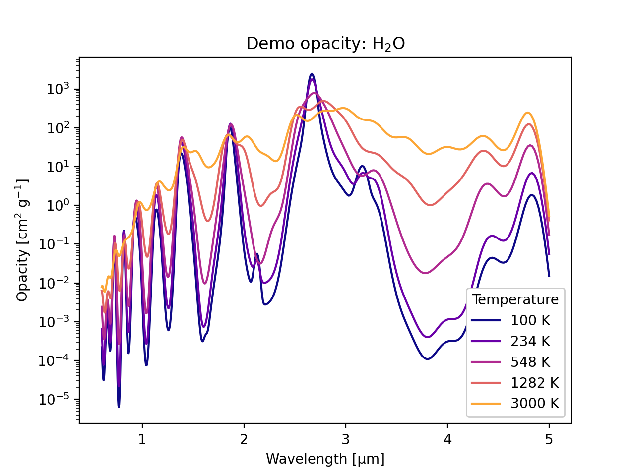
Tiny opacity archives

Warning

These demo opacities are meant for documentation and testing only, and you should not do scientific inference with them. Demos only!

It can be cumbersome to work with opacity grids, given that they may be tens of GB in size. For simple examples in the documentation and tests, shone has very lightweight representations of the full opacity grids for several molecules, which we call “tiny opacity archives”.

To load one of these example opacities, run:

from shone.opacity import Opacity
import numpy as np
import matplotlib.pyplot as plt

# load the tiny opacity archive:
tiny_opacity = Opacity.load_demo_species('H2O')

After you load them, these opacity files work just like the real ones. We can interpolate the grid at several temperatures and plot the results like this:

# get a jitted interpolator:
interp_opacity = tiny_opacity.get_interpolator()

# get opacity at several temperatures, all at 1 bar:
wavelength = np.geomspace(0.6, 5, 500)  # [µm]
temperature = np.geomspace(100, 3000, 5)  # [K]
pressure = np.ones_like(temperature)  # [bar]

kappa = interp_opacity(wavelength, temperature, pressure)

# plot the opacities:
n = len(temperature)
ax = plt.gca()

for i in range(n):
    color = plt.cm.plasma(i / n)
    label = f"{temperature[i]:.0f} K"
    ax.semilogy(wavelength, kappa[i], label=label, color=color)

ax.legend(title='Temperature', loc='lower right', framealpha=1)
ax.set(
    xlabel='Wavelength [µm]',
    ylabel='Opacity [cm$^2$ g$^{-1}$]',
    title="Demo opacity: H$_2$O"
)

(Source code, png)